Prediction using Linear Regression based on First Principles
Published:
Background
Despite the widespread usage and knowledge of linear regression as a machine learning technique for prediction/classification problems, we have found that proper implementation in Python remains scarce among popular, open-sourced libraries. Most libraries encourage a direct application of datasets into a linear model, without explicitly having checks on linear regression assumptions, nor do they provide any understanding of the need for any data transformations, or confidence intervals of projected results.
Hence, we built a lightweight Python module to evaluate datasets on their appropriateness for linear regression and perform necessary transformations. The objective is to generate a forecast within the sample space, with confidence intervals. Here we focus on the use case of Simple Linear Regression, with only one independent variable and one dependent variable.
Procedure
- Download training data from Kaggle: Predicting House Prices
- Plot relevant charts to evaluate core assumptions of linear regression
- Perform statistical tests where relevant, such as the Durbin-Watson Test to check for Independence of Errors
- Analytically compute linear regression coefficients, standard error of regression, mean, and standard errors of coefficients
- Plot Forecast within sample space of training set, and introduce 95% confidence interval
Implementation
First, we perform checks on the core linear regression assumptions of Linearity between variables, Normality of Error Distribution, Independence of Errors, and Homoscedasticity, and obtain the following charts:
Figure 1: Checking on Linear Regression Assumptions
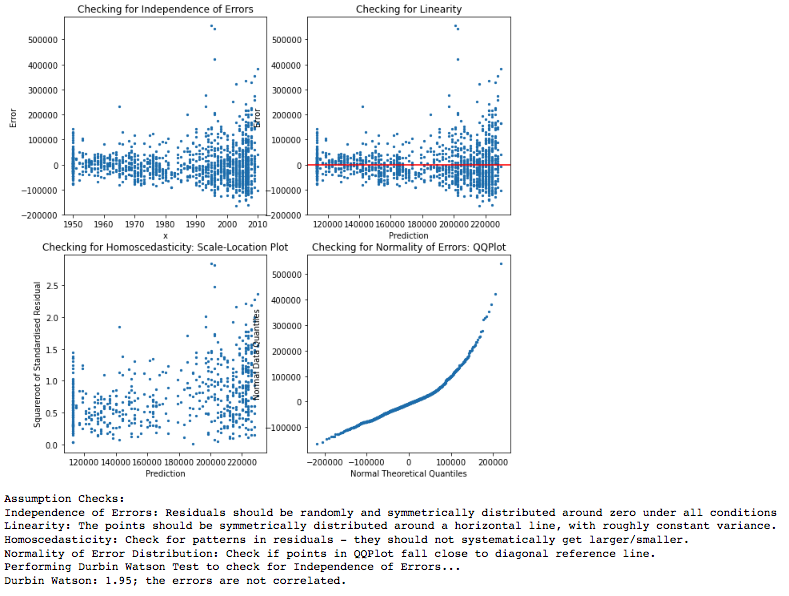
Checking on Assumptions
The module automatically generates the expected distributions of scatter points in each plot, which we will re-iterate below:
- Independence of Errors: In the Residual-independent variable plot, the scatter points should be randomly distributed and symmetically distributed around residual = 0 under all conditions. Additionally, we also check on the Durbin-Watson Score: A score between 1.5 and 2.5 means we can assume that the errors are not correlated.
- Linearity: In the residual-prediction plot, we want to check that the points are symmetrically distributed along the residual = 0 line, with roughly constant variance. A systematically-increasing/decreasing variance may indicate a non-linear relationship. This plot also allows us to check for homoscedasticity.
- Homoscedasticity: We check on the Scale-Location Plot, which is a plot of square-root standardised residuals against prediction. The standardised residuals should not systematically increase in any direction, indicating a constant variance.
- Normality of Error Distribution: We generate a Quantile-Quantile Plot (QQPlot) from first principles, comparing the actual percentile with the theoretical percentiles of a normal distribution. If the QQ Plot is close to a 45 degree line, this means that the error distribution more closely resembles a theoretical normal distribution.
Linear Regression Parameters
In this example we aim to use the ‘Year of Remodelling’ as a predictor for Sale Prices. We perform a log-transformation of sale prices to correct for some heteroscedasticity observed at the right-end of the distribution, which implied an exponential increase in sale prices in the more recent years. After performing the linear regression, we obtain the following parameters:
Figure 2: Fitted Linear Regression Parameters
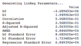
Data Transformation
Based on the assumption check plots above, we see some evidence of heteroscedastcity, as well as non-linearity from the residual-prediction plots. This prompts a log-transformation of the dependent variable. The linear regression coefficients also had very large standard errors, indicating a high level of uncertainty on the coefficients calculated. We re-run the assumption checks after performing the log transformation to obtain the following charts.
Figure 3: Checking on Linear Regression Assumptions (After Log Transformation)
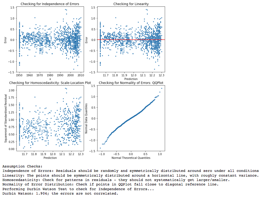
Figure 4: Fitted Linear Regression Parameters (After Log Transformation)
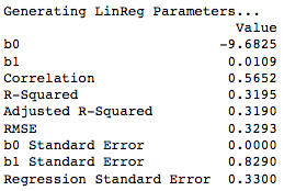
We can observe that performing the log-transformation has increased the adjusted R-squared, and has drastically reduced the standard errors of the linear coefficients.
Forecast
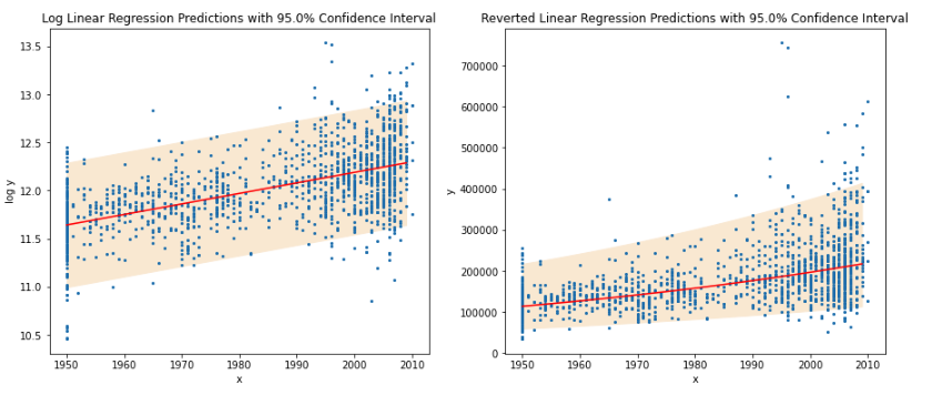
After performing linear regression on the Log of the Sale Price, we obtain linear regression forecasts both in log(price) and price. Sale price projections were generated after applying an exponential to the forecasted log(prices). We compute the 95%s confidence intervals at each sample space by taking the product of the standard error of the forecast (consisting of the standard error of the regression and standard error of the mean at each point), as well as the Critical Z-Value for the 95% significance level. This provides lower and upper boundaries reflecting the confidence interval at each value of the independent variable.
Figure 5: Linear Regression Forecast
Limitations
The objective of this module is to evaluate an independent variable against a dependent variable based on first principles, but uses only a single predictor. More features, and thus multiple-linear regression, should be used to obtain better results, especially with the House Prices Dataset on Kaggle that was used.
Contact
I hope you have enjoyed reading the above piece of analysis. You can refer to the published module on Github.
